Camera Simulation on 3D Data

I used third party ply_read() Matlab function to read the 3D data. I simulate the camera by changing the camera position and rotation in predefined trajectories.

Matlab Code

% USE THIRD PARTY FUNCTION TO READ 3D DATA
[Tri, Pts] = ply_read('bunny.ply', 'tri');
[elements, var] = ply_read('bunny.ply');
conf = elements.vertex.confidence;

c = size(Pts, 2); % NO OF VERTICES
f = 0.05; % F = 50mm
cam_pos = [0; 0; -0.5];
theta_x = 0; theta_y = 0; theta_z = 0;  % CAMERA ROTATION PARAMETERS
video_im = uint8(zeros(301, 301, 1, 301)); % OUTPUT IMAGE FRAMES

% MOVE CAMERA TOWARDS OBJECT IN SINE TRAJECTORY
dist1=-0.5 + sin(linspace(0,pi,100))/10; 
dist4=-0.5 - sin(linspace(0,pi,200));
% ROTATE 360 DEGREES WITH RESPECT TO Y AXIS
dist2=linspace(0,2*pi,200);
% ROTATE 360 DEGREES WITH RESPECT TO X AXIS
dist3=linspace(0,2*pi,200);
% CONCATINATED LIST
dist=[dist1,dist2,dist3];

for i = 1 : length(dist)
% CHANGE TRANSFORMATION PARAMETERS
    if(i <= length(dist1))
        cam_pos=[0;0;dist(i)];
    elseif(i <= length(dist2) + length(dist1))
        theta_y = dist(i);
    else
        theta_x = dist(i);
        theta_y = dist(i);
        theta_z = dist(i);
        cam_pos=[0;0;dist4(i-300)];
    end
% CAMERA TRANSOFRMATION MATRIX (ROTATION)
    Rx = [1 0 0; 0 cos(theta_x) -1*sin(theta_x); 0 sin(theta_x) cos(theta_x)];
    Ry = [cos(theta_y) 0 sin(theta_y); 0 1 0; -1*sin(theta_y) 0 cos(theta_y)];
    Rz = [cos(theta_z) -1*sin(theta_z) 0; sin(theta_z) cos(theta_z) 0; 0 0 1];

    eff_obj_data = Pts - repmat(cam_pos, 1, c);
    D = Rx * Ry * Rz * (eff_obj_data);
    
% APPLY TRANSFORMATION
    P = [f*eye(3) zeros(3,1)]; % CAMERA MATRIX
    im = P*[D; f*ones(1, c)];
    scaled_im = im(1 : 2, :);
    % SCALING THE IMAGE TO THE RANGE
    scaled_im(1, :) = (im(1, :)  - min(im(1, :)))./abs(im(3, :)).*600;
    scaled_im(2, :) = (im(2, :)  - min(im(2, :)))./abs(im(3, :)).*600;
    scaled_im = ceil(scaled_im) + 1;

% INTENSITY MAPPING
    im_out = zeros(301, 301);
    for j = 1 : c
        if(scaled_im(2, j) < 302 && scaled_im(1, j) < 301)
            im_out(302 - scaled_im(2, j), scaled_im(1, j)) = conf(j);
        end
    end
% COLLECTING FRAMES
video_im(:, :, :, i) = uint8(im_out.*200);
end

mov = immovie(video_im, gray);
movie2avi(mov, 'out.avi'); % SAVE VIDEO
implay(mov);

Output

Graph Cut Segmentation

Here, I've used the Planar Graph Cut library on Prof. Olga Veksler's website to develop this program to segment an image using graph cuts.

OpenCV Code

#include "stdafx.h"
#include "windows.h"
#include "CutSegment.h" //include PlanarCut
#include <iostream>
#include <stdio.h>
#include <string>
#include <fstream>
#include <sstream>
#include <stdlib.h>

using namespace std;

unsigned char *loadSimplePPM(int &w, int &h, const string &filename) {
  char line[1000];
  int depth = 0;
  unsigned char *rgb = 0;
  long lastpos;
  FILE *fh = fopen(filename.c_str(), "rb");  
  w = 0, h = 0;
  fgets(line, 1000, fh);
  if (strcmp(line, "P6\n")) {
    cerr << filename << " ist keine PPM-Datei\n";
    return false;
  }
  while (!feof(fh)) {
    lastpos = ftell(fh);    
    fgets(line, 1000, fh);
    if (line[0] == '#') {
    } else if (!w) {
      if (sscanf(line, "%d %d", &w, &h) < 2) {
cerr << "Fehler beim Auslesen der Datei " << filename;
cerr << " Breite und Hoehe des Bildes erwartet\n";
return 0;
      }
    } else if (!depth) {
      if (sscanf(line, "%d", &depth) < 1) {
cerr << "Fehler beim Auslesen der Datei " << filename;
cerr << " Farbtiefe erwartet\n";
return 0;
      }
    } else {
      rgb = new unsigned char[w*h*3];
      fseek(fh, lastpos, SEEK_SET);
      fread(rgb, 1, w*h*3, fh);
      break;
    }  
  }
  fclose(fh);
  return rgb;
}

bool saveSimplePPM(unsigned char *rgb, int w, int h, const string &filename) {
  ofstream fos(filename.c_str(), ios_base::binary);
  ostringstream ost;
  string s;
  if (!fos)
    return false;
  fos << "P6" << endl;
  ost << w << " " << h << endl;
  fos << ost.str();
  fos << "255" << endl;
  fos.write((const char*)rgb, w*h*3);
  fos.close();  
  return true;
}

unsigned char *RGBDataToGrey(unsigned char *rgb, int w, int h) {  
  unsigned char *pic = new unsigned char[w*h];
  int i;
  for (i=0; i<w*h; i++)
    pic[i] = rgb[i*3];
  return pic;
}

unsigned char *GreyDataToRGB(unsigned char *pic, int w, int h) {
  unsigned char *rgb = new unsigned char[w*h*3];
  int i;
  for (i=0; i<w*h; i++)
    rgb[i*3] = rgb[i*3+1] = rgb[i*3+2] = pic[i];  
  return rgb;
}

unsigned char *SegMaskAndGreyDataToRGB(CutPlanar::ELabel *mask, unsigned char *pic, int w, int h) {
  unsigned char *rgb = new unsigned char[w*h*3];
  int i;
  for (i=0; i<w*h; i++) {
    rgb[i*3] = (mask[i]==CutPlanar::LABEL_SINK) ? (unsigned char)(pic[i*3] / 255.f * 200.f) : 255;
    rgb[i*3+1] = (unsigned char)(pic[i*3+1] / 255.f * 200.f);
    rgb[i*3+2] = (mask[i]==CutPlanar::LABEL_SINK) ? 255 : (unsigned char)(pic[i*3+2] / 255.f * 200.f);
  }  
  return rgb;
}

unsigned char *getSegmentationInfo(unsigned char *rgb, int w, int h) {
  unsigned char *seginfo = new unsigned char[w*h];
  unsigned char r, g, b;
  int i;
  for (i=0; i<w*h; i++) {
    r = rgb[i*3];
    g = rgb[i*3+1];
    b = rgb[i*3+2];
    if (r >= 240 && g <= 10  && b <= 10) {
      seginfo[i] = 1;
    } else if (r <= 10 && g <= 10 && b >= 240) {
      seginfo[i] = 2;
    } else {
      seginfo[i] = 0;
    };
  }    
  return seginfo;
}

int _tmain(int argc, _TCHAR* argv[]) {
  CutSegment *sc;
  int w, h;
  uchar *seg, *rgb, *rgbNew, *grey;
  CutPlanar::ELabel *mask;
  size_t pos;
  string picname, segname, basename, suffix;
  char tmp[4096]; //just needed for windows character conversion  
  picname = "F:/PlanarCut/examples/pics/walk1.ppm";
  pos = picname.rfind(".ppm");
  if (pos == string::npos) {
    cerr << "testCutGrid only accepts .ppm images\n";
    return -1;
  }
  suffix = picname.substr(pos);
  basename = picname.substr(0, pos); 
  picname = basename + suffix;
  segname = basename + "seg" + suffix; 
  //load the prelabeled image from file
  rgb = loadSimplePPM(w, h, segname);
  seg = getSegmentationInfo(rgb, w, h);
  delete [] rgb;
  //load the image to be segmented from file
  rgb = loadSimplePPM(w, h, picname);
  grey = RGBDataToGrey(rgb, w, h);
  cout << "Image width: " << w << " and image height " << h << endl;
  //perform segmentation task
  sc = new CutSegment(w, h);
  sc->setImageData(grey);
  sc->setSourceSink(seg,1,2);
  cout << "Cut: " << sc->segment() << "\n";
  mask = new CutPlanar::ELabel[w*h];
  sc->getLabels(mask);
  delete sc;
  //read out segmentation result and save to disk
  rgbNew = SegMaskAndGreyDataToRGB(mask, rgb, w, h);
  saveSimplePPM(rgbNew, w, h, string("segresult.ppm"));
  //release memory
  delete [] grey;
  delete [] rgb;
  delete [] rgbNew;
  delete [] seg;
  delete [] mask;
  return 0;
}

Input

Image to be Segmented

Pre-labeled Image

Output

Segmentation Result

Region Growing

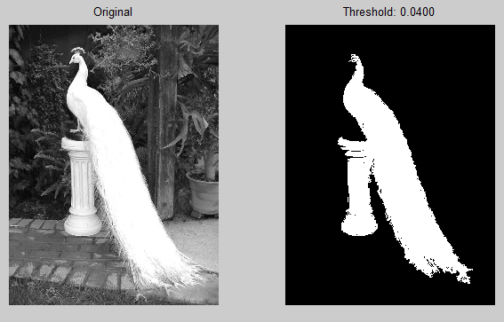
This method gets image and threshold as arugments and gets the mouse click coordinates as the seed to proceed. Here, starting from the seed the intensity values of each pixel is compared with its neighbours and if it is within the threshold, it'll be marked as one.

Matlab Code

function regionGrowing(name,T)
    im=rgb2gray(imread(name));
    im=im2double(im);
    [r,c]=size(im);
    A=zeros(r,c); % segmented mask
    F=[]; % frontier list
    subplot(1,2,1);
    imshow(im);
    title('Original');
    s=uint16(ginput(1));    % get the click coordinates
    s=[s(2),s(1)];      % [row,col]
    A(s(1),s(2))=1;
    F=[F;s];
    while(~isempty(F)) % if frontier is empty
        n=neighbours(F(1,1),F(1,2),r,c);   % 4 neighbourhood
        for i=1:size(n,1)
            if(abs(im(F(1,1),F(1,2))-im(n(i,1),n(i,2)))<T && A(n(i,1),n(i,2))~=1)% less than threshold & not already segmented
                A(n(i,1),n(i,2))=1;
                F=[F;n(i,1),n(i,2)];
            end
        end
        F(1,:)=[];
    end
    subplot(1,2,2);
    imshow(A);
    title(sprintf('Threshold: %0.4f',T));
end

function out=neighbours(s1,s2,r,c)
    out=[];
    if(s2>1),  out=[out;s1,s2-1];   end
    if(s1>1),  out=[out;s1-1,s2];   end
    if(s1<r),  out=[out;s1+1,s2];   end
    if(s2<c),  out=[out;s1,s2+1];   end
end

Output

The segmented region is shown in white.

Gaussian Smoothing

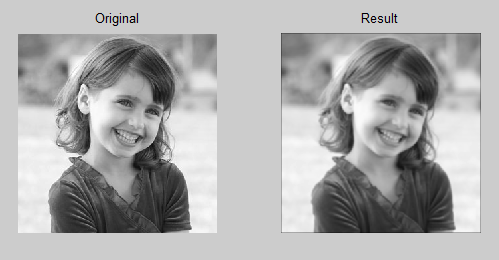
This code takes image name and the kernel size as arguments and does Gaussian smoothing by creating a Gaussian kernel of specified size and apply the kernel to the image.


The output will be a blurred image.


Matlab Code

function gaussianSmoothing(name,w)
    h = gaussianKernel(w); % w x w Gaussian kernel    
    imrgb = imread(name);
    im = im2double(rgb2gray(imrgb));
    result = conv2(im,h,'same'); % Apply the kernel
    subplot(1 ,2 ,1)
    imshow(im);
    title('Original');
    subplot(1 ,2 ,2)
    imshow(result)
    title('Result');
end


function h=gaussianKernel(w)
    x=-floor(w/2):floor(w/2);
    y=-floor(w/2):floor(w/2);
    [X,Y]=meshgrid(x,y);        
    Z=(1/2*pi)*exp(-(X.^2+Y.^2)/2); % sigma=1
    h=Z/sum(sum(Z)); % normalize
end

Output

Gamma Correction

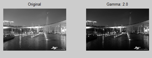
This method takes the image name, c and gamma as arguments and apply the transformation 
s = cr^gamma to each of the pixels and produce the output.


You can note that for gamma > 1, wide range of dark input pixels are mapped into narrow range of output pixels, image will be darkened. Opposite is true for gamma < 1.

Matlab Code

function gammaCorrection(name, c, gamma)
r = imread (name);
r=im2double(r);
r=rgb2gray(r);
s = c * (r .^ gamma);
subplot (1 ,2 ,1)
imshow(r);
title('Original');
subplot (1 ,2 ,2)
imshow(s)
title(sprintf('Gamma: %0.1f',gamma));
end

Output

Zoom Images : Nearest Neighbour & Bilinear Interpolation

The method zoom() will get the image name and the zoom factor as arguments and produce the required zoomed image using both Nearest neighbour and Bilinear interpolation methods to help us compare the results.

In nearest neighbour method, I just repeated the rows and columns to get the required zoom level. 

In bilinear interpolation method, first I copied the original pixel values to a new matrix and did the interpolation in two steps. First, I interpolated the columns (in x-direction) using original pixel values. Then, I interpolated the rows (in y-direction) which finished the bilinear interpolation.

Matlab Code

function zoom (name,n)
    close all
    im=imread(name);
    im=rgb2gray(im);
    imshow(im);
    [r,c]=size(im);
    % NEAREST NEIGHBOUR
    x=zeros(r*n,c*n);
    for i=1:r
        for j=1:c
            x(i*n-n+1:i*n,j*n-n+1:j*n)=repmat(im(i,j),n,n);
        end
    end
    figure
    subplot (1 ,2 ,1)
    imshow(mat2gray(x));
    title('Nearest Neighbour');
    % BILINEAR
    im = im2double(im);
    [r,c]=size(im);
    y=zeros(r*n-n+1,c*n-n+1);
    % COPY THE ORIGINAL VALUES
    for i=1:r
        for j=1:c
            y(i*n-n+1,j*n-n+1)=im(i,j);            
        end
    end         
    % INTERPOLATE IN X-DIRECTION
    [row,col]=size(y);
    for i=1:n:row
        for j=1:col
            m=mod(j,n);
            if(m==0)
                m=n;
            end
            if(m~=1)
                y(i,j)=((m-1)*y(i,j-(m-1)+n) + (n-(m-1))*y(i,j-(m-1)))/n;
            end
        end
    end      
    % INTERPOLATE IN Y-DIRECTION
    for i=1:row
        for j=1:col
            m=mod(i,n);
            if(m==0)
                m=n;
            end            
            if(m~=1)
                y(i,j)=((m-1)*y(i-(m-1)+n,j) + (n-(m-1))*y(i-(m-1),j))/n;
            end
        end
    end
    subplot (1 ,2 ,2)
    imshow(y);
    title('Bilinear');
end

Output

You can notice that, bilinear interpolation method gives more smooth output.